

Several of CVEP’s team members often work remotely. I really like the people I work with, and sometimes I miss our all-hands impromptu discussions around the copier. Often, a topic would come up, or a question, and I would run to my office and quickly produce a map or chart to further our discussion. Now those ad hoc ideas are frequently shared by email.
Our CEO Emeritus, Joe Wallace, likes data as much as I do. He’ll see something on the web that catches his eye and will share it with us. Recently, he saw some data comparing, by state, the percentage of the population with high school degrees or higher. He was dismayed that California is dead last at 82.9% of the population with high school degrees or higher. We follow Mississippi (83.9%) and Texas (83.2%). Who’s at the top? Montana (93.2%), Minnesota (93%), and New Hampshire (92.9%).
But an average percentage belies underlying demographic disparities. And that is what we will look at today. We will compare census data for the US, California, Riverside County, and the nine Coachella Valley cities. We will dig into the data aggregated by age and race/ethnicity.
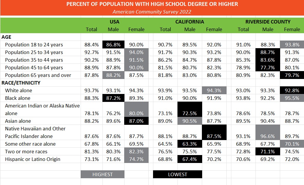
This table compares population proportions of those with high school degrees or higher between the US, California, and Riverside County. The gray boxes show the highest percentages between all three for each age range or race/ethnicity. The black boxes show the lowest concentrations. Every geography has highs and lows.
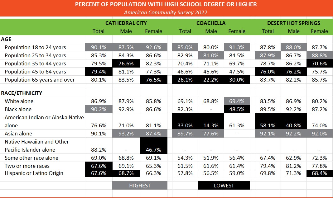
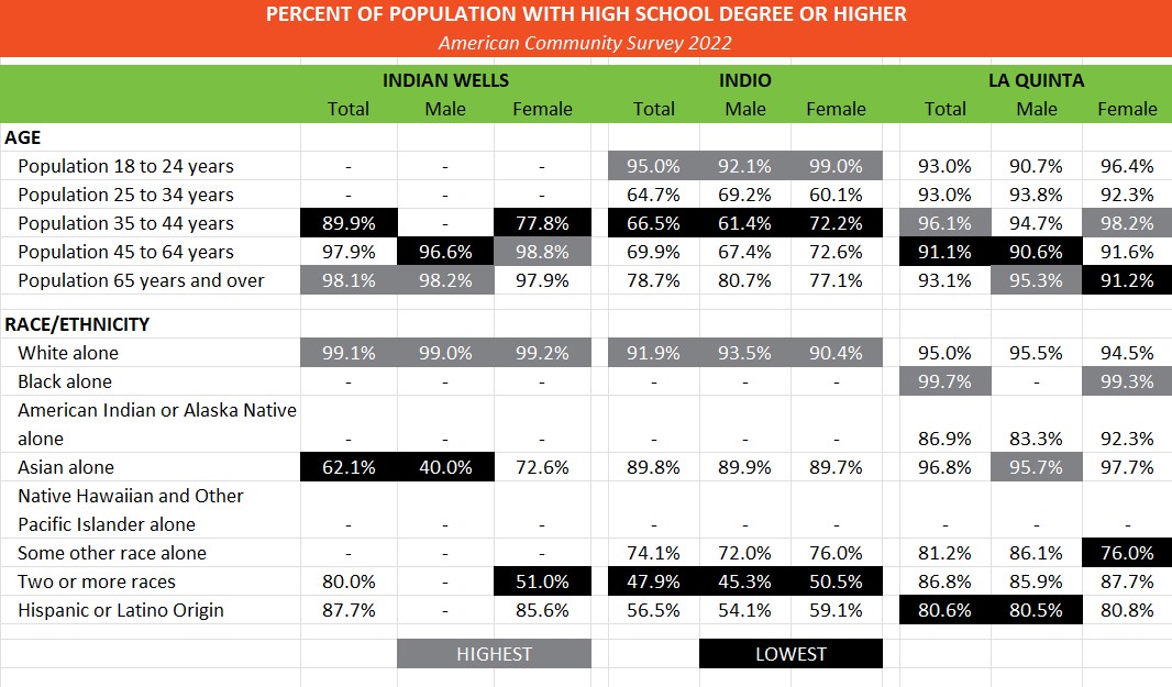
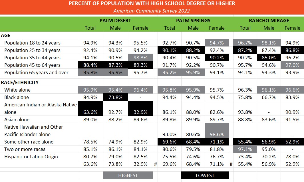
These three tables show concentrations for each of the nine Coachella Valley cities. Note that all of these data are from the American Community Survey. ACS data is collected between each decennial census. The US Census Bureau randomly surveys throughout these 9 years on many topics, including educational attainment. As such, the values in these tables are statistical estimates and can have significant margins of error (included with all Census tables). Still, for comparison sake between geographies and cities, they are enlightening. I have removed all estimates that were 100%. This suggests either too small a survey sampling or too small a population of specific age groups or race/ethnicity groups.
In these three tables, I have indicated the highest and lowest values within each city, not between the cities, like in the first table.
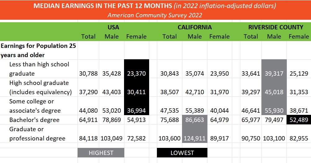
Finally, here we see one of the effects of differential educational attainment. This table shows comparative median earnings by educational attainment. The median highest earners, men with graduate or professional degrees in California, earn over five times that of women with less than a high school degree in the United States.


